Data Science
Inside the Tokeniser: BPE, WordPiece, SentencePiece & Unigram Explained
An example-driven walkthrough of the four major tokenisation algorithms behind modern LLMs, with a step-by-step explanation.
Part 2 of 4 in the "LLM & Tokenization" series
In Tokens 101: The Secret Language Your AI Actually Speaks, we learned that a token can be a word, a sub-word, a character, or a punctuation mark. But who decides where to make the cuts? That's the job of a tokenization algorithm. Different LLMs use different algorithms, and the choice quietly shapes how "smart" the model feels.
Is Tokenisation the Same for Every LLM?
Nope. Every LLM is a bit like a different like appliance in your kitchen a blender, a food processor, a knife each breaks food down differently, even if the end goal (chopped vegetables) is similar. Each LLM (or even different versions of the same LLM) can use a different tokenization algorithm. The vocabulary, the full set of tokens a model knows is essentially known as the model's dictionary.
The bigger and better designed the vocabulary, the more nuance the model can capture. This is why tokenisation isn't a boring technical footnote it's genuinely foundational to how well an LLM understands language.
Why Doesn't an LLM Just Use Normal Human Words as Tokens?
This is a question that must have cross the mind probably for once, and it's exactly what "naive" word-level tokenization tries to do, but with genuinely painful results once you run the numbers.
Imagine treating every word form as its own separate token:
move, moves, moved, moving, mover, movement, movements...
That's already 7 separate vocabulary entries for a single root idea. Now scale that pattern across the English language:
- English has roughly 170,000 words in current use (per the Oxford English Dictionary's count of headwords).
- A typical regular verb has around 5 inflected forms (base, third-person -s, -ing, past tense, past participle). E.x., walk, walks, walking, walked, walked.
- Nouns add plurals, possessives, and compounds. Adjectives add comparatives and superlatives (big, bigger, biggest).
- Add proper nouns, brand names, technical jargon, abbreviations, misspellings, and slang, and realistic estimates for a "cover everything" word-level vocabulary run into the millions of unique entries.
Here's why that is not just "a lot to remember" but actually breaks the model's math. Every single vocabulary entry needs its own embedding vector a list of numbers (say, 768 numbers for a mid-sized model) that represents its meaning. That's stored in a giant lookup table of size vocabulary_size × embedding_dimensions.
Note about embedding vector: An embedding vector is a numerical representation of a piece of text (such as a word, sentence, or document) that captures its semantic meaning. These vectors are stored in a vector database, allowing the system to retrieve text that is semantically similar to a user's query.
Example: "How do I reset my password?" → [0.12, -0.45, 0.78, ...]
When a user asks a question, the question is also converted into an embedding vector. The vector database finds stored vectors that are closest/similar to it, and the retrieved text is then provided to the LLM as context to generate the answer.
| Approach | Vocabulary size | Embedding table size (× 768 dimensions) | Parameters just for this one table |
|---|---|---|---|
| Naive word-level (covers most of English) | ~1,000,000 words | 1,000,000 × 768 | ≈ 768 million parameters |
| Real-world subword tokenizer (e.g., GPT-style) | ~50,000 tokens | 50,000 × 768 | ≈ 38.4 million parameters |
That's roughly a 20x difference and this table has to be duplicated again for the model's output layer (both input and output independently consume parameters ), so the naive approach effectively doubles that burden to over 1.5 billion parameters before the model has done a single bit of "thinking." Worse, most of those million word-entries (rare inflections, one-off brand names, typos) would appear so rarely in training data that the model would barely ever learn anything useful about them you would be paying a massive memory cost for almost no benefit.
This is exactly the problem sub-word tokenization solves. Instead of memorizing "moved" and "moving" as two totally unrelated million-dollar entries, the tokenizer learns to recognize mov as one reusable chunk and glues different, commonly-seen endings onto it (-ed, -ing, -es). Smaller vocabulary, smarter reuse, faster training, and crucially the model can now handle words it has never even seen before by breaking them into familiar pieces.
Subword tokenization is a text-splitting approach where words are broken down into smaller, meaningful chunks called subwords that sit somewhere between individual characters and whole words. Instead of treating every word as one indivisible unit (word-level tokenization) or breaking everything down to single letters (character-level tokenization), subword tokenization finds a middle ground: common words often stay whole, while rarer or more complex words get split into reusable pieces.
For example, the word "unhappiness" might be split into:
[un + happi + ness]
Each piece (un, happi, ness) can be reused across many other words, un also appears in "undo" and "unfair"; ness also appears in "kindness" and "darkness." This reuse is the whole point.
Algorithm #1: Byte-Pair Encoding (BPE)
BPE is one of the oldest tricks in the book (used by GPT-style models), and it's actually simpler than it sounds once you walk through a real example step by step. Here's the idea in plain English first:
- Compute the unique set of words in your training corpus (the "corpus" is just the big pile of text the tokenizer learns from).
- Build a base vocabulary out of every individual symbol (character) used to write those words.
- Split every word into those individual characters.
- Find the most frequently occurring pair of adjacent symbols across the whole corpus.
- Merge that pair into one new, longer token, and add it to the vocabulary.
- Repeat steps 4–5 over and over until you hit your target vocabulary size.
Let's Walkthrouhg the Above with a Practical Example
Say our entire corpus contains just 5 words, and our vocabulary needs to cover them:
hug, pug, pun, bun, hugs
The base vocabulary is simply every distinct character used to spell these words:
["b", "g", "h", "n", "p", "s", "u"] → 7 symbols
(In a real-world tokenizer, this base vocabulary would start with all 256 possible byte values, plus common Unicode characters but 7 is plenty to see how the mechanism works.)
Now let's say these words appear in the corpus with the following frequencies:
- hug: 10
- pug: 5
- pun: 12
- bun: 4
- hugs: 5
Training starts by splitting every word into individual characters, so the tokenizer sees each word as a list of single-character tokens:
- ("h" "u" "g", 10)
- ("p" "u" "g", 5)
- ("p" "u" "n", 12)
- ("b" "u" "n", 4)
- ("h" "u" "g" "s", 5)
At this character-only stage, we can measure two useful numbers:
- Vocabulary size = 7 (just our 7 base characters)
- Total tokens needed to represent the whole corpus = 113 (add up every character across every word, multiplied by how often each word appears)
Now the algorithm looks for the most frequent pair of adjacent symbols. The pair ("h", "u") shows up in "hug" and "hugs" i.e. 15 times total. Not bad, but not the winner. That title goes to ("u", "g"), which appears in "hug", "pug", and "hugs", for 20 times total i.e. the most frequent pair in the corpus.
So the first merge rule the tokenizer learns is: ("u", "g") → "ug". This new token gets added to the vocabulary, and every occurrence of "u" followed by "g" anywhere in the corpus gets merged:
Vocabulary (8): b, g, h, n, p, s, u, ug
Corpus:
- ("h ug", 10)
- ("p ug", 5)
- ("p u n", 12)
- ("b u n", 4)
- ("h ug s", 5)
Tokens needed now: 93, down from 113, just from one merge.
The algorithm repeats: it looks for the next most frequent pair. This time it's ("u", "n"), appearing in "pun" and "bun" for 16 times total. So the second merge rule is: ("u", "n") → "un":
Vocabulary (9): b, g, h, n, p, s, u, ug, un
Corpus:
- ("h ug", 10)
- ("p ug", 5)
- ("p un", 12)
- ("b un", 4)
- ("h ug s", 5)
Tokens needed now: 77.
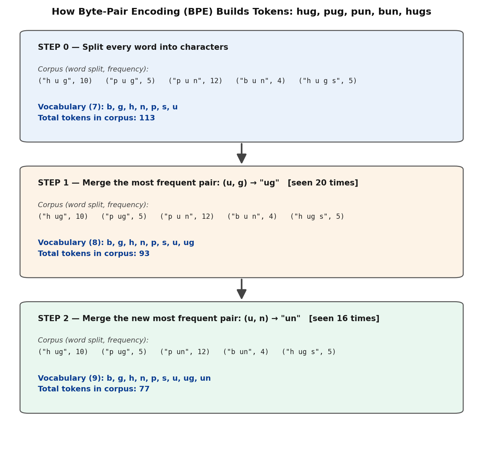 This diagram walks through the exact example above: starting from individual characters, then merging (u,g)→"ug", then merging (u,n)→"un" — with the running vocabulary size and total token count shown at every stage.
Seeing the Compression in Action
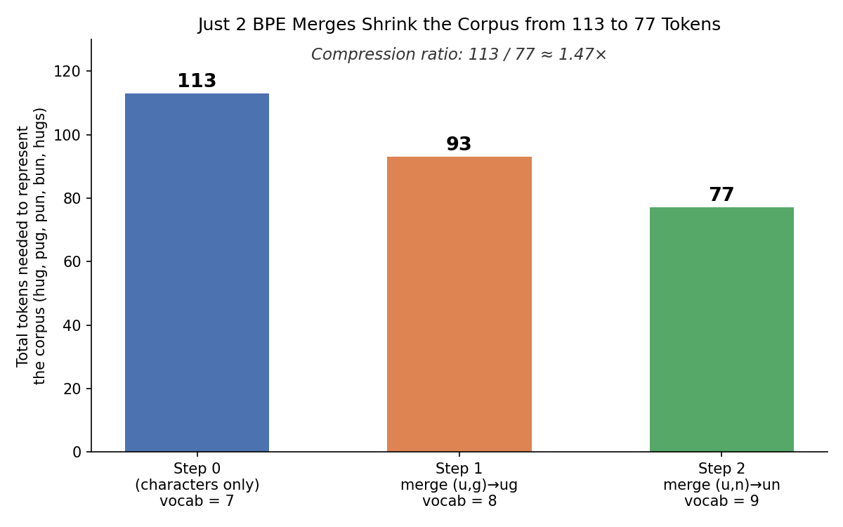 With just 2 merges, the same 36-word corpus needs 77 tokens instead of 113 — a compression ratio of 113 / 77 ≈ 1.47×. Real tokenizers repeat this merge process tens of thousands of times, which is why a production BPE tokenizer (like GPT's, with roughly 50,000 tokens in its vocabulary) can represent huge amounts of text so efficiently.
How to read this chart: Each bar is one stage of training. The height is the total number of tokens needed to represent our fixed 5-word corpus at that stage. As the vocabulary grows by just 2 new tokens (from 7 to 9), the number of tokens needed to write out the same corpus shrinks by 32%. This is the core magic of BPE: a small, smart vocabulary of reusable chunks lets you say the same thing in fewer tokens.
If we kept going, the algorithm would keep hunting for the next most frequent pair perhaps merging ("h", "ug") into "hug" next and repeat this process until it reaches a chosen target vocabulary size. For example, if we wanted a final vocabulary size of 276, we would need to perform 20 total merges on top of a 256-symbol byte-level base vocabulary. Production tokenizers do this same process, just thousands of times over, across billions of words of training text.
Algorithm #2: WordPiece
WordPiece (used by BERT-style models) is BPE's more analytical cousin. BPE's merge rule is simple: whichever pair shows up together most often wins. WordPiece asks a smarter question: instead of raw frequency, it merges the pair that most improves the likelihood of the training data basically, "which merge makes my statistical model of language happiest?"
The formula WordPiece uses to score each candidate pair looks like this:
score(pair) =

frequency(pair) / (frequency(first symbol) × frequency(second symbol))
This normalization is the whole trick. It means WordPiece isn't impressed by a pair just because both halves are common it specifically rewards pairs where the two pieces are individually rare, but frequently seen together, since that combination carries more "surprise value" and is more likely to represent a genuinely meaningful unit.
A Numeric Example
Suppose our training corpus gives us these candidate merges:
| Candidate pair | Pair frequency | freq(first) | freq(second) | Score = pair / (first × second) |
|---|---|---|---|---|
| ("t", "he") | 5,000 | 20,000 | 15,000 | 5,000 / 300,000,000 ≈ 0.0000167 |
| ("un", "able") | 30 | 1,000 | 800 | 30 / 800,000 ≈ 0.0000375 |
Even though ("t", "he") shows up in the corpus 166 times more often in raw terms, ("un", "able") wins the merge because both "un" and "able" are individually much rarer so their strong tendency to appear together is statistically more meaningful. BPE, using raw frequency alone, would have picked ("t", "he") without a second thought. WordPiece specifically avoids merging common filler combinations and prioritizes pairs that behave like a genuine linguistic unit.
The practical result: WordPiece tends to produce sub-words that feel a bit more "linguistically sensible" things like un + ##able, photo + ##graph, or un + ##happiness. It marks word-continuation pieces with a special ## prefix, so the model can always tell "this piece continues the previous word" apart from "this piece starts a brand-new word." For example, the word "unhappiness" might get tokenized as:
un + ##happi + ##ness
Algorithm #3: SentencePiece
SentencePiece isn't exactly a separate merging strategy the way BPE and WordPiece are, it's more of a clever front-end wrapper that fixes a very practical, very common problem: what do you do with languages that don't use spaces between words at all, like Japanese, Thai, or Chinese?
The Whitespace Problem
Traditional tokenizers (including plain BPE and WordPiece as originally described) quietly assume a first step that most people never think about: split the raw text on whitespace first, and then tokenize each resulting word into sub-word pieces. That works fine for English, where words are neatly separated by spaces. It completely falls apart for a language like Japanese, where sentences are written with no spaces between words at all.
Take this real Japanese sentence, meaning "I like cats":
私は猫が好きです
There is no whitespace anywhere in that line for a traditional tokenizer to split on. A word-boundary-first approach simply has no starting point.
How SentencePiece Solves It
SentencePiece skips the whitespace-splitting assumption entirely. It treats the entire raw input including spaces themselves as just another stream of characters to learn from, and then runs a sub-word algorithm (usually BPE or Unigram, the ones we're covering in this article) directly on that raw stream.
To keep track of where spaces originally were (so text can be perfectly reconstructed later), SentencePiece replaces each space with a special visible meta-character, commonly written as ▁ (an underscore-like symbol). For example, the English sentence:
Hello world
gets pre-processed into:
▁Hello▁world
and might then be tokenized into pieces like:
▁Hello ▁world
Each token that starts with ▁ tells the model "this piece began right after a space in the original text" which means the tokenizer can convert tokens back into perfectly-formatted original text, spaces and all, with zero ambiguity. For our Japanese example, since there were no spaces to begin with, SentencePiece would instead lean on its underlying algorithm (often Unigram) to find sensible splits directly from the raw character stream, something like:
▁私 は 猫 が 好き です
— breaking the sentence into meaningful chunks ("I", topic marker, "cat", subject marker, "like", polite verb ending) without ever needing spaces to guide it.
Algorithm #4: Unigram Language Model
Unigram flips the entire process on its head. BPE and WordPiece both build up they start tiny (individual characters) and merge their way up to bigger tokens. Unigram does the opposite: it starts big with a huge pool of candidate sub-words, and prunes down to a final vocabulary by repeatedly removing whichever tokens hurt the model's overall likelihood score the least.
How It Actually Works, Step by Step
- Build a large seed vocabulary. Start with a huge candidate list of sub-words often generated by running BPE first, or simply extracting every frequent substring from the training corpus. This might be tens of thousands of candidate tokens, far more than the final target size.
- Assign each candidate token a probability, estimated from how often it would be used across the corpus, using a statistical technique called Expectation-Maximization (EM) think of it as repeatedly refining a best guess until the numbers stabilize.
- For every word, find its best segmentation, the way of splitting that word into vocabulary tokens that has the highest combined probability (this search is done efficiently with an algorithm called Viterbi, commonly used in speech and language processing).
- Measure how much each token matters. For every candidate token, calculate how much worse (statistically) the corpus would be explained if that token were removed and words had to be re-segmented without it. This "damage score" is called the token's loss.
- Prune the least useful tokens. Remove the bottom 10–20% of tokens with the smallest loss (the ones that barely matter), and repeat the whole process.
- Stop once you hit your target vocabulary size.
A Worked Example
Take the made-up but illustrative word "unaffordable." There are multiple ways a vocabulary could segment this word:
| Candidate segmentation | Illustrative probability of this exact sequence |
|---|---|
un + afford + able | P(un) × P(afford) × P(able) = 0.02 × 0.004 × 0.05 = 0.000004 |
una + fford + able | P(una) × P(fford) × P(able) = 0.0001 × 0.0002 × 0.05 = 0.000000001 |
u + n + a + f + f + o + r + d + a + b + l + e | product of 11 individual character probabilities each small, so the total is astronomically smaller still |
Unigram computes (approximately) all plausible segmentations like this and picks the one with the highest overall probability, in this case, un + afford + able wins by a wide margin, because it's built from chunks that are individually common and combine in a way the model has seen work well before. This is also why Unigram-based tokenizers can gracefully handle a word being split more than one valid way depending on context, rather than being locked into one fixed rule the way BPE's merge list is.
Because it's a probability-based, prune-from-the-top method rather than a fixed merge-list, Unigram (usually paired with SentencePiece as its front-end, since it also needs a way to handle raw, unsegmented text) tends to produce a more flexible, statistically grounded vocabulary one built by asking "how much does the model actually lose without this token?" rather than "how often did I see this pair?"
Quick Comparison Table
| Algorithm | Direction | Used By (style) | Key Trait |
|---|---|---|---|
| BPE | Builds up from characters via frequency | GPT-style models | Simple, fast, frequency-driven |
| WordPiece | Builds up via likelihood score | BERT-style models | Slightly more "linguistically aware" merges |
| SentencePiece | Wrapper (uses BPE or Unigram inside) | Multilingual models | Works on raw text, no whitespace assumption |
| Unigram | Prunes down from a large candidate pool | Often paired with SentencePiece | Flexible, probability-based token choice |
Example: Same Product Name, Different Tokenizers
Consider a fictional fashion e-commerce brand, UrbanTrend, selling a product called "Re-Stitch Denim Jacket."
- A BPE-based assistant might tokenize it as:
Re-StitchDenimJacket - A WordPiece-based assistant might tokenize it as:
Re##StitchDenimJacket - A Unigram-based assistant might instead choose:
Re-StitchDenimJacket(treating the hyphenated term as a single learned chunk, if it appeared often enough in training)
UrbanTrend's data team noticed that product titles with unusual hyphenation or invented brand words (like "Re-Stitch") consumed noticeably more tokens on some models than others a small detail that quietly affected their AI-powered product-description generation costs at scale.
Key Takeaways
- Tokenization isn't one universal method it's an algorithm, and different LLMs pick different ones.
- BPE merges the most frequent character pairs, bottom-up.
- WordPiece merges the pair that most improves statistical likelihood.
- SentencePiece is a wrapper that tokenizes raw text directly, ideal for languages without spaces.
- Unigram starts big and prunes down to the most useful sub-words.
- The choice of algorithm shapes a model's vocabulary, and vocabulary is the foundation of understanding.
Up next in Part 3: We tackle token limits what happens when your input is simply too big for the model to handle, using a regression-model analogy that will make it click instantly.
In case of any queries or feedback feel free to drop comments or reach out using the Contact secion.