Data Science
The Brier score: Helps in Model Evaluation for Probabilistic Classifiers
A working example of the Brier score, why it punishes confident wrong answers, and how it helps in model comparison, calibration, and monitoring.
What is the Brier score?
The Brier score measures how close a model's predicted probabilities are to what actually happened. For a single prediction, it is the squared difference between the predicted probability and the real outcome, where the outcome is coded as 1 if the event happened and 0 if it did not:
error = (predicted probability − actual outcome)²The Brier score for a whole dataset is the average of that error across every prediction:
Brier score = (1 / N) × Σ (pᵢ − yᵢ)²
pᵢ - predicted probability for the i case
yᵢ - actual outcome (1 or 0) for the i case,
N - total number of cases.- It ranges from 0 to 1 for a binary outcome.
- Score of 0 means every prediction was exactly right
- Score of 1 means every prediction was fully confident and fully wrong.
- Lower brier score is always better.
The metric is named after Glenn Brier, a meteorologist who proposed it in 1950 to grade weather forecasts. A forecaster who says "70% chance of rain" is making a probabilistic claim, and Brier wanted a way to check whether those percentages held up over many days. The same question applies to almost every classification model built today.
Why is it needed?
Most classification models output a probability, then we often throw that information away. Accuracy, precision and recall only look at which side of a threshold the prediction landed on. ROC-AUC looks at whether positives were ranked above negatives. None of these checks whether a prediction of 0.30 actually corresponds to a 30% chance.
That gap matters whenever the probability itself drives a decision:
- An insurer prices a policy using the predicted probability of a claim.
- A bank sets credit limits from the predicted probability of default.
- A marketing team multiplies purchase probability by order value to estimate expected revenue per customer.
- A hospital flags patients whose predicted risk of readmission crosses 20%.
In each case a model can rank cases well and still give numbers that are systematically too high or too low. The property being tested here is called Calibration. Among all the cases where the model predicted 30% probability, about 30% should turn out positive. The Brier score is sensitive to both ranking quality and calibration at once, which is why it catches problems that ranking metrics miss.
A worked example with four predictions
Take a model that predicts whether a customer will make a purchase, and look at four customers:
| Customer | Predicted probability | Actual outcome | Squared error |
|---|---|---|---|
| A | 0.9 | Bought (1) | (0.9 − 1)² = 0.01 |
| B | 0.1 | Did not buy (0) | (0.1 − 0)² = 0.01 |
| C | 0.7 | Did not buy (0) | (0.7 − 0)² = 0.49 |
| D | 0.3 | Bought (1) | (0.3 − 1)² = 0.49 |
Brier score: (0.01 + 0.01 + 0.49 + 0.49) / 4 = 0.25.
A and B were predicted well. A 90% prediction that came true and a 10% prediction that did not come true both produce a tiny error. C and D were predicted with fair confidence in the wrong direction, and they account for almost all of the score. Two good predictions and two poor ones average out to 0.25 because the confident misses dominate.
For reference, a model that predicts 0.5 for everything also scores 0.25 on any dataset. So this example model, despite getting half the cases nearly right, is no better than a coin flip on this metric.
How to read the chart
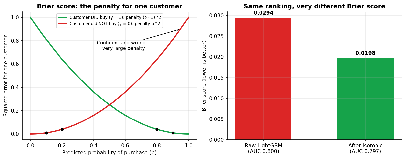
Figure 1. Left: the Brier penalty for a single prediction. Right: the Brier score of the same model before and after calibration.
Left chart: the penalty for one prediction
The x-axis is the predicted probability, and the y-axis is the squared error that one prediction adds to the score. There are two curves because the penalty depends on what actually happened:
p is predcted probability, y is actual outcome (1 or 0).
- The green curve applies when the event happened (y = 1). The penalty is (p − 1)², so it is 1.0 at p = 0 and falls to 0 at p = 1. Predicting high is rewarded.
- The red curve applies when the event did not happen (y = 0). The penalty is p², so it starts at 0 and climbs to 1.0 at p = 1. Predicting low is rewarded.
The black dots mark predictions of 0.1, 0.2, 0.8 and 0.9 that turned out correct,they all sit near the floor, with penalties of 0.01 or 0.04.
The curves are bowls, not straight lines, and that shape is the main thing to take from the panel. Going from 60% to 90% confidence on a wrong prediction raises the penalty from 0.36 to 0.81, more than double. Small errors are cheap and confident errors are expensive. The two curves cross at p = 0.5 with a penalty of 0.25, which is the most a forecaster can lose by saying "I don't know."
This shape also makes the Brier score a proper scoring rule. The expected penalty is lowest when the model reports its honest probability. Rounding a 70% belief up to 95% to look decisive, or squashing it toward 50% to play safe, both increase the expected score.
Right chart: same ranking, different Brier score
The right chart compares two versions of the same gradient-boosted model (LightGBM) on a purchase dataset:
| Version | Brier score | ROC-AUC |
|---|---|---|
| Raw LightGBM | 0.0294 | 0.800 |
| After isotonic calibration | 0.0198 | 0.797 |
ROC-AUC barely moves, from 0.800 to 0.797, so both versions rank customers almost identically. The Brier score falls by about a third. The only change between the two bars is calibration: isotonic regression was fitted on held-out data to map the raw scores onto probabilities that match observed purchase rates.
Interpretation: When two models have nearly the same AUC but very different Brier scores, the difference is almost entirely calibration. The model with the lower Brier score is the one whose probabilities you can use directly in a calculation.
Brier Skill Score
A raw Brier score is hard to judge alone, because its scale depends on how common the event is. With rare events the numbers are always small. In the dataset behind the chart, only 2.38% of customers bought. A model that ignores every feature and predicts 2.38% for everyone has a Brier score of:
baseline_brier = base_rate * (1 - base_rate)
               = 0.0238 * (1 - 0.0238) = 0.0232
Now the chart's numbers have context:
| Model | Brier score | Beats the baseline? |
|---|---|---|
| Always predict the base rate | 0.0232 | n/a |
| Raw LightGBM | 0.0294 | No, worse by about 27% |
| LightGBM after isotonic calibration | 0.0198 | Yes, better by about 15% |
The raw model, with a respectable 0.80 AUC, scores worse than a model that looks at nothing. This is common with models trained using class weights or oversampling to handle imbalance: those techniques help ranking but inflate the predicted probabilities. Once calibrated, the same model beats the baseline.
The relative improvement over the baseline is called the Brier skill score:
brier_skill_score = 1 - (model_brier / baseline_brier)- A positive(+ve) value means the model adds information beyond the base rate.
- Zero(0) means no skill
- Negative(-ve) value means the probabilities are worse than not having a model.
For the calibrated model above it is 1 − 0.0198 / 0.0232, about 0.15.
When to use and not to use the Brier score
When to use
The Brier score is for classification problems where the model outputs a probability and that probability will be used as a number. It fits best when:
- Decisions use expected values, such as probability times revenue, loss or cost.
- Several models feed one downstream system that assumes they speak the same probability language.
- The threshold may change later, so you care about the whole probability scale and not one cut-off.
- Stakeholders read the score directly ("this patient has a 15% risk").
Typical applications include credit default and probability-of-default models, insurance claim prediction, churn and purchase propensity, fraud scoring, click-through rate prediction in advertising, clinical risk scores, demand forecasting of yes/no events, and sports or election forecasting.
When not to use
- It is not meant for regression problems with a continuous target.
- It is a poor choice when we need only a ranked list and will never use the probabilities as numbers. There, ROC-AUC, precision-at-k or lift answer the question more directly.
Which kind of model use Brier score most often
Any model that produces class probabilities can be scored with brier. The metric is most useful for model families known to drift away from good calibration:
- Gradient-boosted trees (XGBoost, LightGBM, CatBoost) are usually well ranked but can be miscalibrated, especially with class weights, heavy regularisation or early stopping tuned on AUC.
- Random forests tend to pull probabilities toward the middle and rarely predict values close to 0 or 1.
- Deep neural networks, particularly large modern ones, are often overconfident.
- Naive Bayes pushes probabilities toward the extremes because of its independence assumption.
- Support vector machines do not output probabilities at all without an added step such as Platt scaling, and that step should be checked.
- Logistic regression is often reasonably calibrated by construction, so it makes a good reference point, though it can still be off when the model is misspecified or the data has shifted.
How it is used in practice
- Model selection: Report the Brier score next to ROC-AUC or PR-AUC on the same validation set. Use AUC to judge ranking and Brier to judge whether the probabilities are usable.
- Checking calibration methods: Fit Platt scaling or isotonic regression on a held-out set, then compare Brier scores before and after, as in the right panel of Figure 1. In scikit-learn,
CalibratedClassifierCVdoes the fitting andbrier_score_lossdoes the scoring. - Baseline check: Always compute the Brier baseline and the Brier skill score. If the model does not beat the baseline, fix calibration before anyone uses its probabilities.
- Pairing with a reliability diagram: The Brier score tells you there is a calibration problem. A reliability diagram (predicted probability buckets against observed rates) shows where it is, for example "overconfident above 0.6."
- Monitoring in production: Track the Brier score on recent labelled data over time. A rising score with flat AUC is an early sign that the base rate has shifted and the model needs recalibration, even if retraining is not yet needed.
A minimal example in Python:
from sklearn.metrics import brier_score_loss

y_true = [1, 0, 0, 1]
y_prob = [0.9, 0.1, 0.7, 0.3]

print(brier_score_loss(y_true, y_prob))  # 0.25
Limitations to keep in mind
- With rare events the scores are tiny and the differences between models look small. Use the skill score rather than the raw number when reporting to stakeholders.
- It treats all errors symmetrically. If a false negative costs far more than a false positive, a cost-weighted metric may suit the decision better.
- It combines calibration and discrimination in one number. Two models with the same Brier score can fail in different ways, so pair it with AUC and a reliability diagram.
- Log loss is a stricter alternative that punishes confident wrong answers much more heavily, without limit as the prediction approaches 0 or 1. Brier is more forgiving of the occasional extreme miss, which makes it easier to read and less sensitive to a handful of outliers.
Key takeaways
- The Brier score is the average squared gap between predicted probabilities and actual outcomes. Lower is better, and confident wrong predictions dominate it.
- It is a proper scoring rule, so it rewards honest probabilities over confident-looking ones.
- A model can have strong ROC-AUC and a poor Brier score at the same time. That combination points to miscalibration.
- Always compare Brier score against the baseline. If the model cannot beat it, its probabilities should not be used as numbers.
- Use it for any probabilistic classifier whose outputs feed pricing, expected value, risk thresholds or reporting, and especially for boosted trees, random forests and neural networks, which often need calibration.
Full code: A simple implementation of the Brier Score using the same data behind the Purchase Propsenity model is available on GitHub.