Analytics
Synthetic Control: Result Validation with RMSPE and Placebos
Part 2 of 3: validate a Synthetic Control result with RMSPE, the RMSPE ratio, placebo tests, plus the Python code that fits the weights.
Jargon check
- Counterfactual: What would have happened without the campaign. The synthetic city is our estimate of it.
- Pre-launch fit: How closely the synthetic city tracks the real city before launch. A good fit is the reason to trust it after launch.
- RMSPE (Root Mean Squared Prediction Error): A general-purpose measure of how far predictions are from reality, in the same units as the thing you predict. Formula:
RMSPE = sqrt( (1 / T) × Σ (Actual_t − Predicted_t)² ), where T is the number of weeks and Σ means "add up over every week t". In words: take each week's error, square it, average the squares, then take the square root. Squaring stops plus and minus errors from cancelling and makes big misses count more; the square root brings the answer back to sales units. In this series "Predicted" is the synthetic city. Example: errors of +1, -1, +2, -1, -1 give an RMSPE of 1.26, so the model usually misses by about Rs 1.3 lakh a week. Smaller means a better fit.- RMSPE ratio: Post-launch RMSPE divided by pre-launch RMSPE. A ratio of 8.5 means the gap after launch is 8.5 times the normal weekly miss. A big number points to a real effect.
- p-value: The chance of seeing a result this extreme if the campaign did nothing. Smaller is stronger evidence.
- Holdout: Weeks set aside from fitting, used only to test whether the model predicts well.
- Weights: The percentages of each donor city used in the blend. They are zero or more and add up to 100%.
In Part 1 - Synthetic Control: The Core Idea our virtual Pune said free delivery earned Rs 32 lakh, an 8.8% lift. A Chief Data Officer (CDO) may ask the next question: "How do you know that is real and not random noise?"
There are 2 ways to answer it:
- RMSPE checks how good the virtual city is.
- Placebo tests check whether your gap is unusual.
How RMSPE Works
The formula itself is simple: actual minus synthetic. Validation uses a different calculation.
RMSPE (Root Mean Squared Prediction Error) is the typical size of the model's miss in a normal week. Find each week's error, square it, average the squares, take the square root.
| Week | Actual | Synthetic | Error | Error squared |
|---|---|---|---|---|
| W1 | 101 | 100 | +1 | 1 |
| W2 | 99 | 100 | -1 | 1 |
| W3 | 112 | 110 | +2 | 4 |
| W4 | 110 | 111 | -1 | 1 |
| W5 | 119 | 120 | -1 | 1 |
| Average of squares | 1.6 |
Square root of 1.6 is 1.26. The single control city from Part 1 scores 2.14 by the same maths, so the synthetic version is about 40% more accurate before launch.
For leadership, convert it: 1.26 divided by the average weekly sales of 108.2 (This is Pune's average weekly sales over the five pre-launch weeks: (101 + 99 + 112 + 110 + 119) ÷ 5 = 108.2) is about 1.2% (1.26/108.2). A good rule of thumb is anything below 5% is good.
The RMSPE ratio: is the gap real?
| Measure | Value | Meaning |
|---|---|---|
| Pre-launch RMSPE | 1.26 | Normal noise when nothing is happening |
| Post-launch RMSPE | 10.7 | Size of the gap after launch |
| Ratio (post / pre) | 8.5 | The gap is 8.5 times normal noise |
| Ratio | How to read it |
|---|---|
| Around 1 | No effect |
| 2 to 3 | Weak signal, check placebos |
| 5 or more | Strong signal, likely real |
Furthermore run a holdout check i.e. fit on weeks 1 to 44, then test on weeks 45 to 52, which are still pre-launch. If the model cannot predict untreated weeks, it cannot be trusted on treated ones or actual production launch analysis.
The Placebo test
A placebo test works like this: "If I pretend a city that got nothing was treated, do I also see a big effect?"
You run it for every donor city, not just one. With 25 donors, that means 25 placebo runs.
- Take each donor city in turn and pretend it was the test city.
- Build its synthetic version from the other 24 donors (the 25 donors minus the city you are pretending is treated, since a city cannot be its own donor). The real test city is never used, because it really was treated.
- Compute each city's RMSPE ratio. That gives 25 placebo ratios plus the real test city's ratio, 26 in total.
- Rank the real test city among all 26.
The 24 donors in step 2 only describe how each single placebo is built. The ranking in step 4 always uses all 26 ratios (25 placebos plus the real test city), so the p-value is out of 26, not 25. Only the real test city gets a p-value. The placebo ratios are the reference for what chance looks like.
The p-value is the test city's rank divided by the total number of cities, which is the number of donors plus one:
p = rank / (number of donors + 1)
If the test city ranks 1st, then p = 1 / (25 + 1) = 1/26, about 0.04. If it ranked 3rd, p would be 3/26, about 0.12. In the chart below (simulated Pune-like city, 25 donors), the test city ranks 1st of 26.
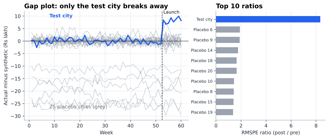
Simulated run: A Pune-like test city and 25 donors, so 25 placebo cities (grey). The blue test city breaks away after launch. The placebo cities do not.
How to read the Chart
Left Chart
- X axis: week. Y axis: actual minus synthetic. Near zero means the model predicts well.
- Grey lines: placebo cities. They wiggle around zero because nothing happened to them. A few sit lower because they are poorly matched.
- Blue line: the test city. It is near zero before launch and breaks away after.
Right Chart
- The 10 largest RMSPE ratios. Blue is the test city.
With 10 donors the lowest possible p-value is 1 / (10 + 1), about 0.09. With 25 donors it is 1 / (25 + 1), about 0.04. More donors means finer inference. In general practice it is wise to drop placebos that fit very badly before launch, because their ratios are meaningless.
Additional methods to check for robustness
- In-time placebo. Assume the campaign started 10 weeks earlier. Using only pre-launch data check the metrics and we shouldn't see any difference in RMSPE.
- Leave one out. Remove the top-weighted donor and refit. The lift should barely move. If it vanishes, then it means one city carries wighs in on the result.
The Python code
The core idea is a small optimisation: weights of at least zero, summing to 1, with the smallest squared error before launch.
import numpy as np
from scipy.optimize import minimize

def fit_scm_weights(y_test_pre, Y_donors_pre):
    n = Y_donors_pre.shape[1]
    loss = lambda w: np.sum((y_test_pre - Y_donors_pre @ w) ** 2)
    res = minimize(loss, np.ones(n) / n, method="SLSQP",
                   bounds=[(0, 1)] * n,                                        # no negatives
                   constraints={"type": "eq", "fun": lambda w: w.sum() - 1})   # sum to 100%
    return res.x

def synthetic_control(y_test, Y_donors, n_pre):
    w = fit_scm_weights(y_test[:n_pre], Y_donors[:n_pre])
    synthetic = Y_donors @ w
    return w, synthetic, y_test[n_pre:] - synthetic[n_pre:]   # weights, series, lift
They question that may arise is: Why not use ordinary regression? This is so because it could return equation like this "Pune = 2.7 x Nagpur - 1.9 x Indore", which fits the past but is meaningless because you cannot subtract a city. The above two rules keep the synthetic city in a realistic blend.
Note: The 50/30/20 mix was chosen for simplication and understanding. On this tiny 5-week table the optimiser returns about 53/15/32 and a lift near Rs 34 lakh. Both fit well, which shows that few weeks and few donors give unstable weights. When we have 52 or more weeks the weights will settle.
The python code for comparison and all the simulated data is available in this notebook
Key takeaways
- The answer between the test city and its synthetic control is a simple difference.
- RMSPE and placebos tell whether we should believe in the result.
- Pre-launch RMSPE measures fit (aim under 5% of average sales).
- The post/pre ratio measures how unusual the gap is.
- A placebo p-value is the test city's rank divided by the number of cities.
- Add in-time, leave-one-out and holdout checks before coming to a conclusion.
Next: Part 3 - Pitfalls & Limitations.
What pre-launch error would you accept before trusting a test: 1%, 3%, 5%?