Data Science
Population Stability Index (PSI): Spot Model Drift Before Your Metrics Do
What PSI measures, how to compute it bin by bin, the 0.10 and 0.25 rules of thumb, and where it is used in model monitoring, with a worked credit example.
- The Population Stability Index (PSI) measures how far today's scored population has drifted from the one your model was built on
- The usual rule of thumb: PSI below 0.10 is fine, 0.10 to 0.25 deserves a look, and above 0.25 means something has changed.
- PSI needs only scores, not outcomes, so it can warn you months before defaults or churn reveal a problem.
Say you trained an ML model. AUC looked great, the validation report got signed off, and it went live. Fast forward six months: is it still seeing the same kind of data it was trained on?
We often can't answer that with accuracy metrics, because the outcomes (defaults or churn) haven't arrived yet. A loan defaults 12 months after it's booked, and a churned customer only shows up as churned once the quarter closes. PSI gets around the wait by asking a simpler question: Does the score distribution today look like the one at development time? If the population has moved, your model is now working on people (read as different dataset) it never saw in training, and you want to know that before the defaults show up. This is often called population drift or data drift.
How PSI works
We compare two distributions of the same variable, usually the model score:
- Expected (E): the baseline, typically the development or validation sample.
- Actual (A): the recent population we are scoring now, say last month's applicants.
Split the baseline score into bins (deciles are the standard choice), work out the share of each sample in each bin, and add up:
PSI = Σ over bins i of (Aᵢ − Eᵢ) × ln(Aᵢ / Eᵢ)Each term is always zero or positive. (If a bin's share goes up, both parts of the product are positive, and if it goes down, both are negative.(Quick Check box explains this) So shifts never cancel out, and a bin with no change adds exactly zero.
💡 Quick check: A bin that grows from 10% to 15% gives (+0.05) × ln(1.5) = (+0.05) × (+0.405) = +0.020. A bin that shrinks from 20% to 15% gives (−0.05) × ln(0.75) = (−0.05) × (−0.288) = +0.014. One rose and one fell, and both still add to PSI. Note: ln (1) = 0, ln(x<1) = negative, ln(x>1) = positive.
📌 Key idea: PSI measures a change in the inputs the model sees. It says nothing directly about whether the model's predictions are still accurate. A high PSI is a reason to investigate performance, and the investigation still has to happen.
A simple example to illustrate the calculation
Take five score bands. The table below lists the baseline share against this month's share:
| Score band | Expected (E) | Actual (A) | A − E | ln(A/E) | Contribution |
|---|---|---|---|---|---|
| 300–500 | 10% | 15% | +0.05 | 0.405 | 0.0203 |
| 501–600 | 20% | 25% | +0.05 | 0.223 | 0.0112 |
| 601–700 | 40% | 35% | −0.05 | −0.134 | 0.0067 |
| 701–800 | 20% | 15% | −0.05 | −0.288 | 0.0144 |
| 801–900 | 10% | 10% | 0.00 | 0.000 | 0.0000 |
| Total | 100% | 100% | 0.0525 |
A PSI of about 0.05 sits in the stable zone. Notice that the same 5-point move adds more in the 300–500 band (0.020) than in the 601–700 band (0.007), because 5 points is a much bigger relative change on a 10% base than on a 40% one. PSI is most sensitive in the thin bins, and it's worth remembering for when one sparse bin suddenly drives your whole number.
Business Scenario: LendLoop's credit score
LendLoop, a fictional digital lender, scores personal-loan applicants on a 300–900 scale. The baseline is its development sample, cut into ten equal deciles of 10% each. In February 2026 the marketing team launches a campaign aimed at first-time borrowers, many of them with thin credit files.
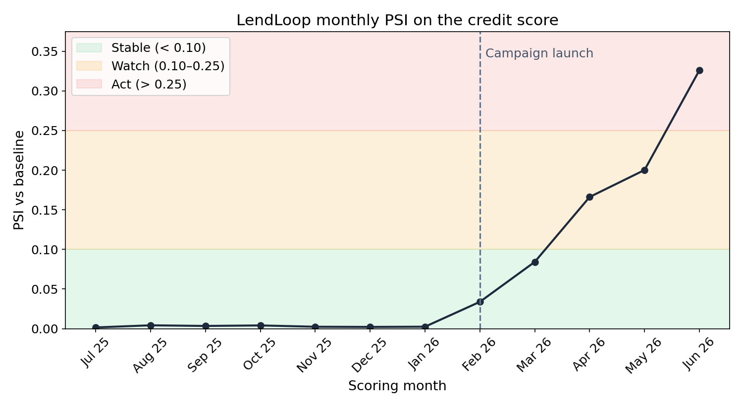
Figure 1: LendLoop's monthly PSI against the development baseline, with the rule-of-thumb bands shaded.
The x-axis shows the scoring month, and the y-axis shows PSI against the baseline. The shaded bands are the usual thresholds: green below 0.10, amber from 0.10 to 0.25, red above 0.25. For seven months PSI barely leaves zero. After the campaign it climbs to 0.08 in March, 0.17 in April, 0.20 in May and 0.33 in June.
A single PSI number tells something moved but not where. Breaking it into per-bin contributions answers the second question.
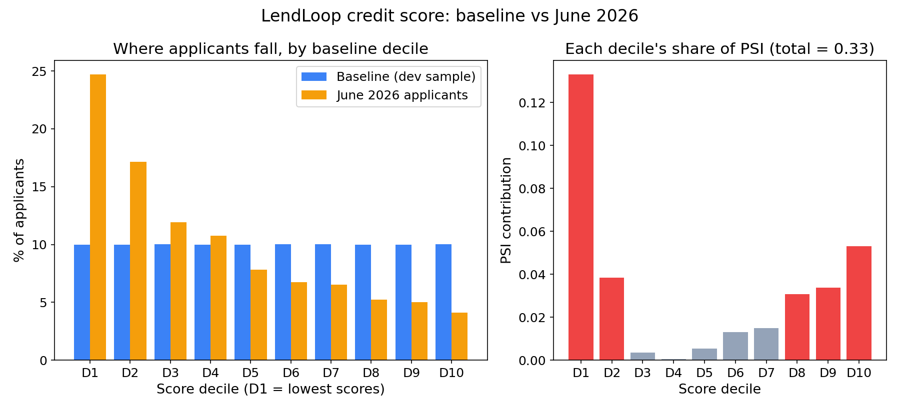
Figure 2: June 2026 score mix against the baseline (left) and how much each decile adds to PSI (right).
The blue bars are all 10% by design: the decile cut points were set on the baseline so each holds exactly a tenth of it. Those same cut points are then reused for June, so any orange bar that isn't 10% shows where the population has moved.
Interpretation of the above Graphs:
- On the left, blue bars are the baseline (10% per decile by construction) and orange bars are June's applicants. D1 is the lowest-scoring decile.
- On the right, each bar is one decile's term in the PSI sum, with red marking the bigger contributors. D1 alone holds 24.7% of June applicants, and it adds 0.13 of the 0.33 total.
- The top deciles drain at the same time, so the whole distribution has slid left. That matches the campaign: more applicants with lower scores.
- This explain that model hasn't broken. It's now scoring a riskier crowd than it was built for, and the cut-offs and expected loss numbers set on the old population need cross checking.
💡 Tip: When the score PSI goes amber, run the same calculation on each input feature. It is called the Characteristic Stability Index (CSI), and it usually points straight at the variable that moved.
To compute it yourself, fix the bin edges on the baseline and reuse them for every later month. Sample code is given below:
import numpy as np

def psi(expected, actual, bins=10, eps=1e-4):
    edges = np.quantile(expected, np.linspace(0, 1, bins + 1))
    edges[0], edges[-1] = -np.inf, np.inf          # catch out-of-range scores
    e = np.histogram(expected, edges)[0] / len(expected)
    a = np.histogram(actual, edges)[0] / len(actual)
    e, a = np.clip(e, eps, None), np.clip(a, eps, None)  # avoid log(0)
    return np.sum((a - e) * np.log(a / e))
Where PSI shows up
Credit risk is where PSI comes from, and it's still a routine line in scorecard monitoring packs and model risk reviews. The same idea carries over to any model that runs in production long before its outcomes are known:
- A fictional retailer, CartNest, tracks PSI on its churn-propensity score after each festive sale, because sale-season shoppers look very different from regulars.
- A fictional insurer, MediSure, runs PSI on its claims-fraud score whenever it adds a new distribution partner.
- Teams with feature stores run CSI on every input weekly and alert when one crosses 0.10.
| PSI | CSI | KS two-sample test | |
|---|---|---|---|
| What it compares | Model score, baseline vs now | One input feature, baseline vs now | Any two distributions |
| Output | One number, rule-of-thumb bands | One number per feature | Statistic plus p-value |
| Works on categories | Yes, each category is a bin | Yes | No, continuous only |
| Watch out for | Bin choice, empty bins | Many features means many alerts | Huge samples make tiny shifts "significant" |
⚠️ Pitfall: The 0.10 and 0.25 cut-offs are industry convention with no statistical test behind them. PSI also creeps up with more bins and with small samples, so keep the binning fixed and don't compare PSI values computed on different setups.
Key Takeaways
- PSI compares the score distribution now with the one at development, bin by bin, and needs no outcome labels.
- Below 0.10 is generally treated as stable, 0.10 to 0.25 as worth a look, and above 0.25 as a real shift. Treat those as conventions.
- Look at per-bin contributions to see where the population moved, then run CSI on features to find out why.
- A high PSI is a prompt to check calibration and cut-offs. It isn't proof that the model is wrong.
Quick Quiz: Test Yourself
1. Why can PSI be monitored before any loan has had time to default?
- A) It uses a proxy default label from the bureau
- B) It only compares score distributions, so no outcome labels are needed
- C) It is computed on the training data only
- D) It estimates future AUC from current scores
Show answer
B. PSI compares how the baseline and current populations spread across score bins. Outcomes never enter the formula, which is what makes it useful early.
2. A bin goes from 10% to 15%, and another goes from 40% to 45%. Which adds more to PSI?
- A) The 10% to 15% bin
- B) The 40% to 45% bin
- C) They add the same, since both moved 5 points
Show answer
A. Both have A − E = 0.05, but ln(15/10) ≈ 0.405 is much larger than ln(45/40) ≈ 0.118. Relative change drives the log term, so thin bins weigh more.
3. LendLoop's score PSI hits 0.33 in June. What is the best next step?
- A) Retrain the model immediately on June data
- B) Ignore it, since PSI says nothing about accuracy
- C) Break PSI down by bin, run CSI on the features, and check calibration and cut-offs on the new mix
- D) Increase the number of bins until PSI drops
Show answer
C. A PSI above 0.25 signals a real shift, so you investigate where and why it moved and whether the model still holds up. Retraining without labels for the new population is premature, and changing bins to lower PSI just hides the shift.
In case of any queries or feedback, feel free to drop a comment or reach out using the Contact section.