Analytics
Synthetic DiD: Working Example With Explanation
Part 2 of 3: The Pune free-delivery example reworked as Synthetic Difference-in-Differences, with time weights explained.
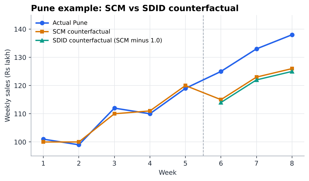
The SDID counterfactual (green) sits 1 unit below the Synthetic Control one (orange).
Jargon check
- Counterfactual: What would have happened without the campaign.
- City weights: The share of each donor city in the blend.
- Time weights: The share of each pre-launch week used as the "before" baseline.
- Intercept: The fixed gap between the test city and the blend, absorbed instead of matched.
- Double difference: The test city's change minus the synthetic city's change. What remains is the campaign.
- Flipped table: The same data turned on its side, with cities as rows and weeks as columns, to find week weights.
- Point estimate: A single best-guess number, with no range around it.
In Part 1 - Core Idea we understood why SDID exists. Now we run it on the same fictional Pune free-delivery data from the Synthetic Control series, so you can check every number by hand.
We keep the city weights at 50% Nagpur, 30% Indore, 20% Surat. A real SDID fit would spread them a little because of the penalty. We add the two other SDID ingredients: an intercept and time weights.
SDID process with example
| Stage | What SDID does | In this article |
|---|---|---|
| 1. City weights | Finds the donor blend that tracks the test city's ups and downs before launch, using an intercept and a ridge penalty | Step 1, Manual calculation, using Synthetic Control's 50/30/20 weights instead of fitted ones |
| 2. Time weights | Finds the mix of pre-launch weeks that best predicts the donor cities' campaign weeks | Step 2. The idea is shown by hand; the 40% / 60% values are illustrative |
| 3. Double difference | Test city's change minus the synthetic city's change, using both sets of weights | Step 3, calculated exactly |
| 4. Counterfactual and lift | Turns the double difference into week-by-week lift | Step 4, calculated exactly |
| 5. Uncertainty | Reruns the estimate many ways (placebo, jackknife or bootstrap) to get a standard error and a confidence interval | Done by code, not by hand. See the note after the Python code |
Stages 1 and 2 are where a real fit would give different weights from our rounded ones. Stages 3 and 4 are the same arithmetic whatever the weights are.
Step 1: City weights and intercept
| Week | Actual Pune | Synthetic | Gap (actual minus synthetic) |
|---|---|---|---|
| W1 | 101 | 100 | +1 |
| W2 | 99 | 100 | -1 |
| W3 | 112 | 110 | +2 |
| W4 | 110 | 111 | -1 |
| W5 | 119 | 120 | -1 |
| Average gap (intercept) | 0 |
The intercept is 0 because Synthetic Pune already matches Pune's level. If Pune was twice the size of every donor, Synthetic Control would fail here, while SDID would simply absorb the difference.
This 0 only confirms that the sizes match. It is not the gap SDID subtracts at the end. That gap comes from the time weights in Step 2 and works out to -1.0 in Step 4. Keep both numbers in mind; the difference between them is what time weights do.
Step 2: Time weights
Time weights answer one question: Which pre-launch weeks look most like the campaign weeks?
To answer it, SDID ignores Pune (its campaign weeks contain the effect) and looks only at the donor cities, which never got the campaign. It flips the table so cities are rows and weeks are columns:
| City | W1 | W2 | W3 | W4 | W5 | Target: avg of W6 to W8 |
|---|---|---|---|---|---|---|
| Nagpur | 110 | 104 | 120 | 116 | 130 | 130.0 |
| Indore | 90 | 100 | 100 | 110 | 110 | 116.7 |
| Surat | 90 | 90 | 100 | 100 | 110 | 106.7 |
| Donor average | 96.7 | 98.0 | 106.7 | 108.7 | 116.7 | 117.8 |
| Distance from target (week avg minus 117.8) | -21.1 | -19.8 | -11.1 | -9.1 | -1.1 | 0 (reference) |
How -21.1 is worked out (W1)
Each target is a donor's average over the three campaign weeks. Nagpur sold 124, 130 and 136, so its target is (124 + 130 + 136) / 3 = 130.0. Indore's is 116.7 and Surat's is 106.7, worked out the same way.
- Solution Process 1, city by city. Nagpur 110 - 130.0 = -20.0. Indore 90 - 116.7 = -26.7. Surat 90 - 106.7 = -16.7. Average: (-20.0 - 26.7 - 16.7) / 3 = -21.1.
- Solution Process 2, averages first. W1 donor average = (110 + 90 + 90) / 3 = 96.7. Target average = (130.0 + 116.7 + 106.7) / 3 = 117.8. Distance = 96.7 - 117.8 = -21.1.
Both processes always give the same number, so the table shows the shorter one.
Interpretation: For the donors, W1 and W2 sit about 20 units below campaign-week sales, while W4 and W5 sit close to them. The recent weeks are the best stand-in for "the campaign period without a campaign", so they get the weight.
| Week | W1 | W2 | W3 | W4 | W5 |
|---|---|---|---|---|---|
| Time weight (illustrative) | 0% | 0% | 0% | 40% | 60% |
Time weights have their own intercept, just like city weights. So strictly, SDID cares less about the raw distance and more about whether a week sits the same distance below the campaign level in every city. W4 is the most consistent (-14, -6.7 and -6.7), which is why the code below leans hardest on W4. We use the rounded 40% / 60% split to keep the arithmetic easy to follow.
Step 3: The double difference
| Weighted "before" (0.4 x W4 + 0.6 x W5) | Average "after" (W6 to W8) | Change | |
|---|---|---|---|
| Actual Pune | 115.4 | 132.0 | +16.6 |
| Synthetic Pune | 116.4 | 121.3 | +4.9 |
| Difference of changes | +11.7 per week |
Over the three campaign weeks that is 11.7 x 3, or about 35. Step 4 gets the same total week by week.
Step 4: Week by week
The counterfactual is Synthetic Pune plus the time-weighted pre-launch gap: 0.4 x (-1) + 0.6 x (-1) = -1.0.
| Week | Actual | Synthetic | Counterfactual | Lift |
|---|---|---|---|---|
| W6 | 125 | 115 | 114 | +11 |
| W7 | 133 | 123 | 122 | +11 |
| W8 | 138 | 126 | 125 | +13 |
| Total | 396 | 364 | 361 | +35 |
| Synthetic Control | Synthetic DiD | |
|---|---|---|
| Baseline | Synthetic city as-is | Synthetic city plus the gap in W4 to W5 |
| Incremental sales | Rs 32 lakh | Rs 35 lakh |
| Lift | 8.8% | 9.7% |
What the time weights changed
Rerun Step 3 with every pre-launch week counted equally (20% each) and compare:
| "Before" weeks used | Pune before | Synthetic before | Difference of changes | Total lift | Lift |
|---|---|---|---|---|---|
| All five, equally | 108.2 | 108.2 | +10.7 per week | 32 | 8.8% |
| Time weights (W4 40%, W5 60%) | 115.4 | 116.4 | +11.7 per week | 35 | 9.7% |
With equal weights the usual gap is the plain average, 0, so SDID gives exactly the Synthetic Control answer. With time weights, only W4 and W5 count, and in those weeks Pune ran 1 unit below its blend. SDID treats that as Pune's normal for this time of year. It lowers the baseline by 1 a week, which credits the campaign with 3 more units over the three weeks.
They agree closely because Synthetic Pune already matched Pune's level. SDID matters most when the test city is much bigger or smaller than the donors, or when recent weeks behave differently from older ones.
Practical Example: SDID edge over SCM
Now make Pune 40 units bigger every week, before and during the campaign: 141, 139, 152, 150, 159, then 165, 173, 178. The campaign is unchanged, so the true extra sales are still 35. Pune is now bigger than every donor in every week.
| Synthetic Control | Synthetic DiD | |
|---|---|---|
| City weights | 100% Nagpur, the highest blend allowed | 50% Nagpur, 30% Indore, 20% Surat |
| Pre-launch gap (W1 to W5) | +31, +35, +32, +34, +29. Never closes | +41, +39, +42, +39, +39. Steady, so the intercept absorbs it |
| Gap added to the baseline | None | +39 (time-weighted: 0.4 x 39 + 0.6 x 39) |
| Counterfactual W6 to W8 | 124, 130, 136 (total 390) | 154, 162, 165 (total 481) |
| Incremental sales | Rs 126 lakh | Rs 35 lakh |
| Lift | 32.3% | 7.3% |
Synthetic Control cannot build anything bigger than Nagpur, so it treats Pune's normal size advantage of about 30 lakh a week as campaign lift and more than triples the answer. SDID does not need the blend to match Pune's size, only its ups and downs. It measures the steady +39 gap before launch, carries it forward, and recovers the same Rs 35 lakh as before. The lift falls from 9.7% to 7.3% only because the same 35 lakh is now measured against a bigger city.
This is the Part 1 problem in miniature: in that simulation Synthetic Control reported 37.9% against a true 8%, and SDID reported 7.9%.
How the weights are found
Both methods are "regression with rules". SDID runs the same weight search three times:
| Search | Table used | Result |
|---|---|---|
| City weights | Weeks as rows, cities as columns | Which cities to blend (with intercept and ridge penalty) |
| Week weights | Flipped: cities as rows, pre-weeks as columns | Which pre-weeks to use as the baseline |
| Final lift | Both sets of weights | Weighted double difference |
The flipped table is the one from Step 2. It asks: "Which blend of pre-weeks looks most like the campaign weeks for these untreated cities?"
The Python code
import numpy as np
from scipy.optimize import minimize

def simplex_least_squares(X, y, ridge=0.0):
    """Weights >= 0 that add to 1, minimising squared error (+ optional ridge)."""
    n = X.shape[1]
    loss = lambda w: np.sum((y - X @ w) ** 2) + ridge * np.sum(w ** 2)
    res = minimize(loss, np.ones(n) / n, method="SLSQP", bounds=[(0, 1)] * n,
                   constraints={"type": "eq", "fun": lambda w: w.sum() - 1})
    return res.x

def synthetic_did(y_test, Y_donors, n_pre):
    pre_d, post_d = Y_donors[:n_pre], Y_donors[n_pre:]
    pre_t, post_t = y_test[:n_pre], y_test[n_pre:]

    # 1. City weights. Centring each series removes the level (the intercept).
    sigma = np.std(np.diff(pre_d, axis=0))
    zeta2 = (len(post_t) ** 0.25 * sigma) ** 2           # ridge strength
    omega = simplex_least_squares(pre_d - pre_d.mean(0), pre_t - pre_t.mean(),
                                  ridge=zeta2 * n_pre)

    # 2. Week weights. Flip the table: cities as rows, weeks as columns.
    X, y = pre_d.T, post_d.mean(0)
    lam = simplex_least_squares(X - X.mean(0), y - y.mean(), ridge=1e-6)

    # 3. Weighted double difference.
    test_change  = post_t.mean() - lam @ pre_t
    synth_change = post_d.mean(0) @ omega - lam @ (pre_d @ omega)
    return omega, lam, test_change - synth_change        # average weekly lift
Compare with Synthetic Control, which is one optimisation on raw levels:
# Synthetic Control: weights >= 0, sum to 1, no intercept
minimize  sum( (test - Donors @ w) ** 2 )

# Synthetic DiD: add an intercept w0 and a ridge penalty
minimize  sum( (w0 + Donors @ w - test) ** 2 )  +  penalty * sum(w ** 2)
If the above code is run on the Pune numbers, we will not get the weights used above.
The code returns city weights of about 37% Nagpur, 28% Indore and 34% Surat, and week weights of about 14%, 0%, 14%, 58% and 14% for W1 to W5, with a lift of about 11.75 per week. With only three donors and five pre-launch weeks the search has very little to work with, so small changes in the data move the weights a lot. The working example above uses rounded weights so every step can be calculated by hand. On real data with 20+ donors and 52+ weeks, use the fitted weights.
Key takeaways
- SDID keeps the Synthetic Control blend, adds an intercept, a ridge penalty and time weights.
- The effect is a weighted double difference: the test city's change minus the synthetic city's change.
- In the Pune example SDID gave 9.7% against 8.8% for Synthetic Control. They agree when the level already matches.
- Make Pune 40 units bigger and Synthetic Control reports 32.3% (Rs 126 lakh) while SDID still finds the same Rs 35 lakh. The intercept is what saves it.
- Week weights come from running the same weight search on the flipped table.
Next: Part 3, which method to use and what can go wrong.