Projects
Data Preparation: Cleaning, Sessionizing, and Feature Engineering
Part 3 of 6. How to clean web clickstream data, build sessions, create the target and engineer features that carry purchase intent.
Most of the business value in a propensity model comes from its features. A modest algorithm on good features beats a fancy one on raw events. This article follows Analyst Jack Ryan work from a messy event log to a table a model can learn from. All the code is in the GitHub repo.
Data Understanding - Clickstream or Website Data
Clickstream data records what visitors do on the site, one event per row. A slice for two BrightCart customers:
| Customer | Timestamp | Event | Product | Category | Device |
|---|---|---|---|---|---|
| C001 | Jan 10 | page_view | P100 | Shoes | Mobile |
| C001 | Jan 10 | product_view | P100 | Shoes | Mobile |
| C001 | Jan 11 | add_to_cart | P100 | Shoes | Mobile |
| C001 | Jan 15 | product_view | P200 | Bags | Mobile |
| C002 | Jan 12 | page_view | P500 | Electronics | Desktop |
Typical events include page_view, product_view, search, add_to_cart, remove_from_cart, wishlist, checkout, purchase and login. Useful attributes include customer ID, session ID, product, category, price, device, browser, traffic source, campaign and geography.
Web behavior is one among the several data sources. Telesales notes, CRM history and email engagement can join the same customer table later. For an easy understanding these articles focuses only on web data because it is timely, granular and available for nearly every customer.
Data Cleaning - Before model preparation
Raw website clickstream data is dirty. In the synthetic dataset we deliberately added problems to illustrate the cleaning steps. The real data is usually worse, and the same steps apply. We remove invalid records, align time zones, drop duplicates, filter bot traffic, and sort by customer and timestamp. The cleaned data is ready for sessionization and feature engineering. The data after cleaning has 1,409,817 rows, down from 1,515,570 in the raw file.
| Step | Rows left | Rows removed |
|---|---|---|
| Raw file | 1,515,570 | 0 |
| Drop missing timestamps and invalid customer IDs | 1,506,509 | 9,061 |
| Standardize time zones, then drop duplicates | 1,484,375 | 22,134 |
| Remove bot traffic (25 bot IDs) | 1,409,817 | 74,558 |
-
About 5% of our rows were logged in IST (UTC+5:30), and the same event logged in two zones looks like two events until you align them. Convert to one zone first, then de-duplicate.
-
Bot traffic corrupts the data. 25 fake IDs produced 74,558 events, and left in they would distort every frequency feature. A velocity rule catches them, since no human fires more than 500 events in a day. Finally, sort by
customer_idandtimestampso that everything downstream can rely on order.
Data Preparation - Build sessions
Many logs arrive without session IDs, so we build them from an inactivity threshold, commonly used 30 minutes of inactivity from the first event.
10:01 page_view
10:05 product_view
10:12 add_to_cart
10:18 checkout        -> Session 1

11:05 product_view    -> Session 2 (47 minutes after the last event)
With pandas this takes 4 lines to compute the gap between events, flag new sessions, and assign a session number and ID:
gap = ev.groupby("customer_id")["timestamp"].diff()
new_session = gap.isna() | (gap > pd.Timedelta(minutes=30))
ev["session_no"] = new_session.groupby(ev["customer_id"]).cumsum()
ev["session_id"] = ev["customer_id"] + "_" + ev["session_no"].astype(str).str.zfill(4)
Our cleaned data yields 172,016 sessions averaging 8.2 events each.
Data Preparation - Create the target variable
With a 30-day observation window and a 7-day prediction window, each row gets a label:
| Customer | Observation behavior | Purchase in next 7 days | Target |
|---|---|---|---|
| C001 | High activity | Yes | 1 |
| C002 | Low activity | No | 0 |
| C003 | High activity | Yes | 1 |
| C004 | Medium activity | No | 0 |
We repeat this every Monday, so each Monday is a prediction point T0 and each customer active in the prior 30 days gets one row per T0. Twenty-five Mondays across our 210 days give 184,688 rows, of which 4,209 are buyers (2.28%). Seeing each shopper at several points in their journey gives the model more examples of "about to buy" and "not yet". It also makes rows dependent on each other, which is one more reason to split by time.
Data Preparation - Feature engineering - Create Additional Features
Therea are 7 types of features that can be created with each capturing a different aspect of intent.
| Family | Question it answers | Examples |
|---|---|---|
| Recency | How recently did they act? | days_since_last_visit, days_since_last_cart_add, days_since_last_purchase |
| Frequency | How often? | visits_7d, product_views_30d, searches_30d |
| Engagement | How deeply? | events_per_session, unique_products_viewed |
| Funnel | How far down the journey? | cart_rate, checkout_rate |
| Affinity | What interests them? | views_in_shoes, product_revisit_count |
| Device and channel | How do they arrive? | mobile_ratio, email_ratio |
| Time of week | When do they shop? | weekend_visit_ratio, evening_visit_ratio |
-
Recency and frequency work together. A last product view 2 days ago gives
days_since_last_product_view = 2, and 5 visits with 20 product views in a week givevisits_7d = 5andproduct_views_7d = 20. We compute both 7-day and 30-day counts so the model can see whether interest is speeding up. -
Ratios often say more than counts.
cart_adds / product_viewsdescribes how focused a visit was, and a higher value usually signals stronger intent. 20 product views with 5 cart adds givescart_rate = 5 / 20 = 25%. Repeatedly viewing 1 product is another useful signal, whichproduct_revisit_countandmax_views_same_productcapture.
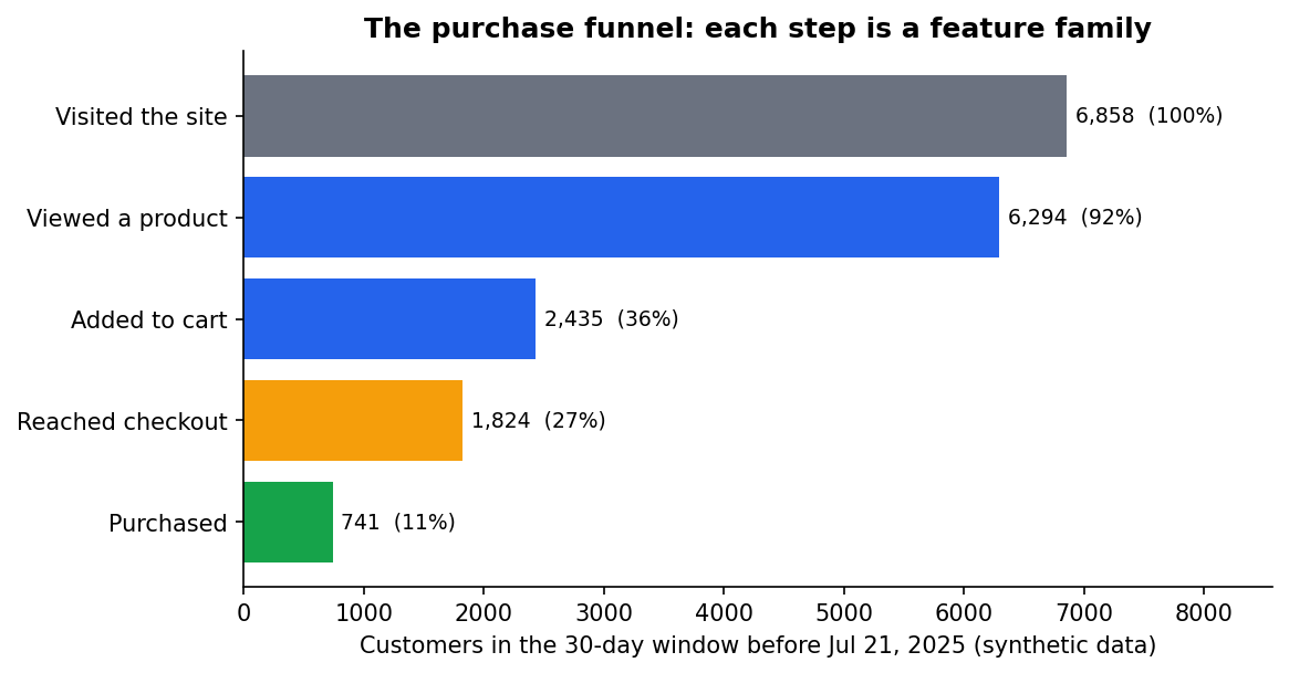
The purchase funnel for BrightCart's active customers in the 30 days before July 21 (synthetic data).
How to read the funnel:
- Each bar counts distinct customers who reached that stage within the 30-day window.
- The percentage is the share of the 7,371 active customers.
- Steep drops mark where intent gets decided. Only 38% add to cart, so cart behavior separates serious shoppers from browsers. The model agrees: how recently a customer last added to cart turns out to be its second-biggest driver, as the SHAP article shows.
Data Preparation Choices - That affect model performance
Both choices below are about features that drift for reasons unrelated to customer behavior. That matters because Part 6 monitors the model for drift.
- Purchase recency (
days_since_last_purchase) looks only inside the observation window. An earlier version of ours looked back through all history, which made the feature depend on how much data each snapshot could see, and the drift check flagged it. tenure_daysis deliberately not a model feature. It grows by one every day for every customer, so it drifts by construction.
Finalised Dataset
The result is a traditional supervised learning table (illustrative rows):
| Customer | recency | visits_7d | product_views | cart_adds | checkout | mobile_ratio | target |
|---|---|---|---|---|---|---|---|
| C001 | 2 | 5 | 20 | 4 | 2 | 0.8 | 1 |
| C002 | 15 | 1 | 2 | 0 | 0 | 0.2 | 0 |
| C003 | 1 | 8 | 35 | 7 | 3 | 0.6 | 1 |
| C004 | 20 | 2 | 4 | 0 | 0 | 0.9 | 0 |
- This is a sample representation of the dataset. This doens't reflect the actual features *
Our real table has 184,688 rows and 50 feature columns. The model uses 49 of them, because
tenure_daysis held out as described above. A quick check shows the signal is there: customers with a cart add in the last 7 days bought in the following week 11.6% of the time, against 1.0% for those without one.
Key takeaways
- Clean the data in order i.e.: invalid records, time zones, duplicates, bots, sort, sessions.
- Build 1 row per customer per prediction date, with features from before T0 and the label from after it.
- Group features into families so you cover different aspects of intent.
- Prefer features that stay stable over time, and drop those that drift by construction.
Part 4 - Model Training focuses to split the data by time, trains three models, and tests them.