Projects
Model Training: Logistic Regression, Random Forest, and LightGBM
Part 4 of 6. Splitting the data by time, training three models of increasing complexity, and reading the first comparison table.
Our smart amazing analyst Jack Ryan created a clean feature table in Part 3 - Data Preparation. The table has 184,688 rows, 50 feature columns, and a target that says whether each customer bought in the 7 days after their prediction date. Training a model on it took less code than everything before it. Judging whether the model could be trusted took longer, and that judgment starts with how the data gets split.
Train-Test Data Splitting - Split by time, not at random
Part 2 - Model Designing suggested an approach for a time-based split instead of a random one. This is how that looks like once we actually draw the line.
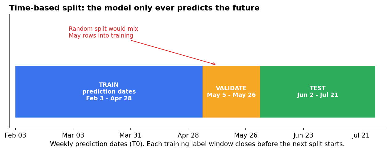
Train on the oldest weeks, validate on the next block, test on the newest. The gap between blocks matters as much as the blocks themselves.
BrightCart's 25 weekly prediction dates split into three groups:
| Split | Prediction dates | Rows | Buyers |
|---|---|---|---|
| Train | Feb 3 to Apr 28 | 95,977 | 2.22% |
| Validate | May 5 to May 26 | 29,536 | 2.28% |
| Test | Jun 2 to Jul 21 | 59,175 | 2.38% |
Training happens once, on the oldest 13 weeks. The model never sees a validation or test row during training, and it never sees a test row until the very end. Every comparison in this article uses the validation set. Test numbers show up in Part 5 - Model Testing and Targeting, the first and only time we look at them.
The validation set is not a "second training set". It's a check on the model's ability to generalize to new data. If the model does well on validation, it has a good chance of doing well on test. If it does poorly, it needs more work before anyone trusts it.
Why there is 7 days gap betwee train and validation, and between validation and test?.
You may notice a 7-day jump between blocks. Training ends on Apr 28 and validation starts on May 5, and validation ends on May 26 and test starts on Jun 2. No week is skipped. We make one prediction every Monday, so every date in the table is simply 7 days after the one before it.
Here is an example with one customer, Carlos:
| Snapshot date | What we do | Block |
|---|---|---|
| Apr 28 | Look at Carlos's activity up to Apr 28, then check whether he buys between Apr 28 and May 5. | Train (last week) |
| May 5 | Look at Carlos's activity up to May 5, then check whether he buys between May 5 and May 12. | Validate (first week) |
Each snapshot asks one question: "will this customer buy in the next 7 days?" The Apr 28 snapshot only checks purchases up to May 5. The May 5 snapshot only checks purchases from May 5 onward. The two checking periods sit side by side and never overlap, so the model is never trained on a purchase that belongs to a validation week. That is why the blocks can touch without leaving a gap between them.
Model Building - Three models, in order of complexity
Jack trained three models so the team could see whether the extra complexity of a modern algorithm was worth it, or whether a simple baseline would have done the job.
-
Logistic regression fits one straight line (in a transformed space) that separates buyers from non-buyers. It is fast, its coefficients are directly readable, and it struggles with features that interact in non-linear ways.
-
Random forest builds many decision trees on random slices of the data and averages their votes. It captures non-linear patterns and interactions without much tuning, at the cost of being harder to explain than a single equation.
-
LightGBM builds decision trees one after another, where each new tree focuses on correcting the mistakes of the ones before it. On tabular data like ours, gradient boosting is usually the strongest of the three, though it needs more care to avoid overfitting.
All three were trained on the same 95,977 rows and the same 49 features (the table has 50 feature columns, but tenure_days is held out, as Part 3 Data Preparation explained), so any difference in their scores comes from the algorithm, not the data.
Data imbalance - How does the model know to care about buyers?
Only 2.22% of the training rows are buyers. That is a problem. A model that predicts "no one will buy" every time would be right about 98% of the time, yet it would never find a single buyer. Part 2 - Model Design warned about the same trap when choosing metrics.
The usual remedy is a class weight. A class weight is a number that multiplies the cost of a mistake for one class. If the weight for buyers is 10, then every time the model misses a buyer, it counts as 10 mistakes instead of 1. The model will try harder to avoid those mistakes, even if it means making more mistakes on non-buyers.
How big should that weight be? There are about 44 non-buyers for every buyer, so the obvious choice is a weight of 44. That makes the buyers, as a group, count as much as the non-buyers.
Two of our models use exactly that. Logistic regression and random forest use scikit-learn's "balanced" setting (the forest uses a per-tree version of it), which works out the 44-to-1 ratio from the training data and applies it for you. We chose it because it is the standard starting point. There is no number to pick, and the right ratio follows automatically if the data changes.
LightGBM is set up differently. It takes the buyer weight as a single number, called scale_pos_weight, so we could choose the value ourselves. We used the square root of 44, about 6.6, as a gentler middle ground between no weight and the full weight. Nothing about the algorithm forces that difference. It is a choice, and it affects the results later in this article.
To see how much the choice matters, we trained each model three times on the training weeks: with no weight, with the square-root weight, and with the full weight. This table shows the average score each version gives on the validation weeks, where the real purchase rate is 2.3%.
| Model | No weight | Square-root weight (6.6) | Full weight (44) |
|---|---|---|---|
| Logistic regression | 2.2% | 10.1% | 35.0% |
| Random forest | 2.2% | 8.7% | 26.9% |
| LightGBM | 2.2% | 8.5% | 26.3% |
The weight moves the scores a lot and the ranking very little. Across all nine runs, ROC-AUC stays between 0.803 and 0.813. PR-AUC drifts in different directions: with the full weight it falls from 0.206 to 0.185 for logistic regression, and rises from 0.222 to 0.229 for random forest and from 0.217 to 0.226 for LightGBM. The average score, by contrast, climbs from 2.2% with no weight to between 26% and 35% with the full weight.
Without any weight, all three models also score a Brier of 0.019 to 0.020, better than the 0.022 of a lazy guess that gives everyone the base rate. The Brier score is explained further down.
So in this data, the weights are not needed to find buyers. The training weeks contain 2,126 buyers, which is enough for these models to learn from on their own. We keep the weights for two reasons. They are widely used in practice, and they matter more when buyers are far rarer than here. And the inflated scores they produce are the problem that Part 5 fixes with calibration.
Treat the weight as a setting to try, not a number to calculate once. Test a few values on the validation data, and judge them by what you need: good ranking, honest probabilities, or both.
Model Results Comparison Table
| Model | ROC-AUC | PR-AUC | Brier | Lift, top 10% | Mean score |
|---|---|---|---|---|---|
| Logistic regression | 0.803 | 0.185 | 0.147 | 6.3x | 35.0% |
| Random forest | 0.805 | 0.229 | 0.088 | 6.6x | 26.9% |
| LightGBM | 0.803 | 0.222 | 0.029 | 6.7x | 8.5% |
Before we pick a winner, let's read the table one column at a time. Each column measures something different, so they can disagree with each other.
ROC-AUC: Can the model put buyers above non-buyers?
Imagine you pick one customer who bought and one who didn't, then ask the model for a score for each. A good model gives the buyer the higher score. ROC-AUC is how often that happens across many such pairs. All three models sit around 0.80, so each one gets the order right about 80% of the time. Because it is so similar for all three, this column can't tell us which model is best. It also tends to look flattering when buyers are rare, because there are so many easy non-buyers to rank below them.
PR-AUC: When the model points at someone, is it right?
Suppose the model flags 100 customers as likely buyers. How many of them really buy? PR-AUC checks exactly this, and it also rewards the model for finding a good share of all the real buyers. This is closer to what a marketing campaign cares about, because every flagged customer costs money to contact. Here the models separate: random forest (0.229) and LightGBM (0.222) both beat logistic regression (0.185).
Brier score: how far are the probabilities from what happened?
For each customer, take the model's score and subtract what really happened (1 if they bought, 0 if they didn't), then square the gap. The Brier score is the average of those squared gaps, and lower is better. ROC-AUC only checks the order of customers. The Brier score checks the numbers themselves. A customer scored 0.90 who doesn't buy costs 0.81. A customer scored 0.02 who doesn't buy costs 0.0004.
A Brier score needs something to be compared with. A lazy model that ignores every feature and gives everyone the base rate (about 2.3%) would score about 0.022 on this validation set. All three of our models score worse than that: 0.147, 0.088 and 0.029. They can still tell buyers from non-buyers, as the ROC-AUC shows. What hurts them is the class weights, which push their scores so far above the real purchase rate that, read as probabilities, they lose to a guess that looks at no customer data at all. LightGBM comes closest because its smaller class weight pushed its scores up the least. The article The Brier score: one number for whether your probabilities can be trusted works through the arithmetic on four customers.
Lift in the top 10%: how much better is the best group than average?
Sort all customers from the highest score to the lowest and take the top 10%. Now compare how many of them buy against the average customer. A lift of 6.7x means they buy 6.7 times as often. With a purchase rate of about 2.3%, that works out to about 15 buyers per 100 customers in the top group, against about 2 per 100 overall. All three models land between 6.3x and 6.7x, so they are about equally good at spotting the very best customers. For this data, the stronger models seem to help more with ordering the customers in the middle of the list than with finding the very top.
Mean score: are the numbers real probabilities?
This column is the average score each model gives. The real purchase rate is only 2.3%, so an honest model should average close to 2.3%. Instead, logistic regression averages 35.0% and LightGBM averages 8.5%. Both are far too high.
This happens because every model here uses class weights, which we added because they are standard practice when buyers are rare. The side effect is that the scores get pushed upward. Think of a weather app that ranks days correctly, with the rainiest days at the top, but says "80% chance of rain" on days when it really rains 20% of the time. The order is right, but the numbers are wrong.
That is fine if all you need is a ranked list ("contact the top 10%"). It becomes a problem when someone reads a score of 0.35 as "this customer has a 35% chance of buying". The article Calibration: turning a ranking into a probability you can actually trust explains how to fix this. In this series the fix is applied at the start of Part 5, before any score is used as a probability.
Reading the precision-recall curves
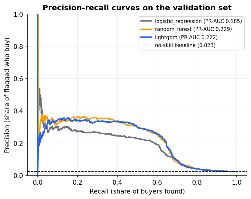
Precision-recall curves on the validation set. Higher and further right is better.
Interpretation of the above chart:
- The x-axis is recall, the share of all real buyers the model would catch if you kept lowering the score cut-off.
- The y-axis is precision, the share of people above that cut-off who actually buy.
- The dashed line at the bottom is what a model with no skill at all would produce, equal to the base rate.
Once past the very top of the ranking, all three curves hold between roughly 0.25 and 0.35 precision over the first 40% of recall, and then fall as you try to catch more buyers, since reaching further down the list always means picking up more false positives. LightGBM and random forest sit clearly above logistic regression through most of the middle range, which is where the PR-AUC gap comes from.
Which model moves forward
Random forest and LightGBM finish almost level on validation. Random forest is a hair ahead on ROC-AUC and PR-AUC (0.805 and 0.229 against 0.803 and 0.222). LightGBM is a hair ahead on lift in the top 10% (6.7x against 6.6x). Gaps this small are not worth arguing over, so the pick is a judgment call: LightGBM is the usual first choice for tabular data, and random forest stays as a close second. The Brier score and average score do not break the tie. LightGBM looks better on both only because it was given a smaller class weight. Give the two models the same weight and their probabilities are about equally far from reality. This was decided on validation data only, and the test set stays closed until Part 5.
Why keep the simple model at all
With both tree models well ahead of it on PR-AUC, it's fair to ask why logistic regression stays in the comparison. Two reasons.
-
- Firstly, It's the model whose coefficients you can read directly, which matters when Opening the black box: explaining the model with SHAP compares three different views of "what matters" and logistic regression is one of them.
-
- Secondly, a small gap between a simple model and a complex one is itself useful information: it tells you the complex model isn't finding some hidden structure the simple one completely misses, just refining an already-clear signal.
What is LightGBM actually using?
LightGBM scores customers well, but 300 trees are not something anyone can read. Before trusting it, Jack asked which features it leans on and whether those make business sense. He used SHAP, a method that splits each customer's score into a push up or down from every feature. The article Opening the black box: explaining the model with SHAP explains how it works.
Averaged over a sample of 4,000 customer-weeks, the three biggest drivers were events per session, days since the last cart add and days since the last product view. Their average pushes were 0.22, 0.16 and 0.13 on the model's internal score scale, well ahead of the 0.09 of the next feature. All three are engagement and recency features from Part 3. That is what a marketer would expect: people who do a lot in each visit, and who touched their cart or a product page recently, are the ones about to buy. It also fits the funnel in Part 3, where only 38% of customers add to cart, which makes a fresh cart add a rare and strong signal.
The same check works as a leakage alarm. A single feature that towered over the rest, or one that could only be known after the prediction date, would send Jack back to the rule from Part 2. The top features here are all computed from events before the prediction date, and the largest push (0.22) is not far above the second (0.16), so nothing points to leakage. SHAP never looks at the purchase outcome, only at the features and the model, so running it on a sample of test customers is not a peek at the test results.
Key takeaways
- Split by prediction date, not randomly, and keep the test set untouched until every other decision is made.
- Class weights fix a model's attention on rare buyers, but they also inflate its raw scores. That trade is fine for ranking and wrong for anything that treats the score as a probability.
- ROC-AUC, PR-AUC, and lift each answer a different question. A model can look identical on one and clearly ahead on another.
- The gap between a simple and a complex model tells you almost as much as either model's individual score.
- The Brier score judges the probabilities themselves, where ROC-AUC and lift judge only the ranking. Against a lazy guess of the base rate for everyone, all three raw models lose, and the class weights are the reason.
- Check what drives the model you carry forward. Here recency and engagement lead, and a check like this doubles as an alarm for leakage.
Part 5 -Model Testing and Targeting opens the test set for the first time: deciles, lift, cumulative gain, calibrating the scores, and turning a ranked list into a campaign audience.