Projects
Model Designing: Observation Window,Populations and Data Leakage
Part 2 of 6 series to explain the problem statement and concept behind Purchase Propensity Model.
Jack Ryan build the requirements from Part 1 - Purchase Propensity Modeling: A Beginner's Guide. Before writing any code she spent 2 days on decisions that no algorithm can make, because each one changes what the model means.
The model at a glance
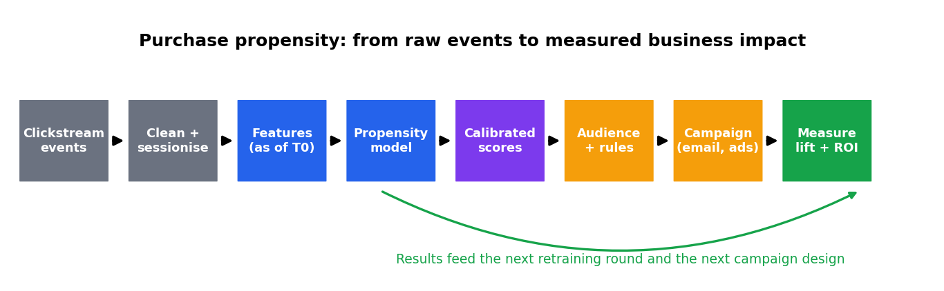
The full journey. Parts 3 to 6 cover each box. Calibration is applied in Part 5 and explained in its own standalone article.
- Raw clickstream events are cleaned and grouped into sessions (Part 3 - Data Preparation).
- Features are computed as of a fixed date and fed to a model (Parts 3 - Data Preparation and 4 - Model Training).
- The raw scores are checked for lift and gain, then calibrated into real probabilities (Part 5). How calibration works is explained in a standalone article, Calibration: turning a ranking into a probability you can actually trust.
- Business rules turn scores into an audience, and the campaign is tested against a holdout (Part 5). Uplift, the production setup and drift monitoring follow in Part 6 - Beyond Propensity Scores.
- Those results shape the next retraining and the next campaign.
The rest of this article covers the choices that sit underneath the above flow.
Prediction Window
The prediction window should match the business action cycle. Ask how far in advance you want to identify a potential buyer. BrightCart sends a campaign every Monday, so the window is 7 days. A monthly campaign would call for 30 days, and a same-day push notification for a few hours. A window longer than the action cycle produces scores that are stale by the time marketing uses them.
Observation Window
Now the next question is how much history helps predict that purchase. Customers have a behavioral memory, and it differs by business. These are 3 fictional examples and their supposed observation period:
| Company | What they sell | Typical research period | Window to test |
|---|---|---|---|
| FreshBasket | Groceries | A few days | 7 to 30 days |
| UrbanNest | Furniture | Several weeks | 60 to 180 days |
| WanderLeaf | Holiday packages | Months | 90 to 365 days |
So "always use 30 days" is a habit, and the right length has to be tested. We rebuilt the BrightCart dataset with four look-backs, trained the same LightGBM model on each, and scored all four on identical customer-weeks. The rows must match, because a shorter window keeps fewer and more active customers, which lifts the base rate on its own.
| Observation window | PR-AUC | Top 10% lift |
|---|---|---|
| 7 days | 0.268 | 6.7x |
| 14 days | 0.263 | 6.8x |
| 30 days | 0.271 | 6.7x |
| 45 days | 0.269 | 6.6x |
The four windows land within noise of each other. That is a legitimate result. In this simulated shop, shopping episodes last a few days by design, so a week of history says as much as six. A furniture retailer would probably see performance keep climbing out to 60 or 90 days.
Two cautions apply. Confirm the choice on several historical splits, because one split can favor a window by luck. And when windows tie, take the shorter one, which needs less history and covers newer customers.
Modeling population and targeting population
Suppose Customer A:
- bought on day minus 20
- viewed a product on day minus 10
- and added to cart on day minus 2.
Should A be in the dataset? Usually yes.
The earlier purchase is historical information available at T0, and features such as days_since_last_purchase = 20 or purchases_last_30d = 1 can be strong signals. Whether A belongs depends on the target definition:
- If the aim is to predict any purchase in the next 7 days, include A.
- If the campaign hunts for first-time buyers, A is out of the eligible population, since that is a different problem.
- In a subscription business, a customer who subscribed yesterday is already a customer, and predicting a new subscription for them makes no sense.
This is why two populations exist:
| Modeling population | Targeting population | |
|---|---|---|
| Question | Who can be in training and scoring? | Who can receive the campaign? |
| Filters | Active in the last 30 days | Also consent, contact frequency, campaign rules |
| BrightCart size (Jul 21) | 7,371 customers | 387 after rules, see Part 5 |
It is better to think like this: "I wouldn't automatically drop customers who purchased during the observation window. A previous purchase is historical information and can be a strong feature. Inclusion depends on the business definition, such as repeat versus first purchase. I would also separate the model population from the campaign-eligible population."
Leakage
Leakage means a feature carries information that would not exist at prediction time. The model looks brilliant in testing and fails in production.
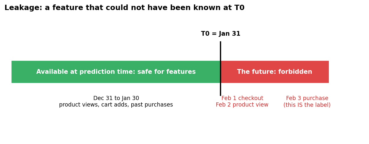
Everything left of the black line is fair game for features. Everything right of it belongs to the future.
With T0 on January 31, a February 1 checkout, a February 2 product view and a February 3 purchase are all off limits as features, and the last one is the label itself. Real leakage is usually quieter:
- A "total purchases to date" column refreshed after the prediction date.
- A customer status field that changes when someone buys.
- A random train and test split that mixes future weeks into training.
The solution is simple. Every feature is computed as of T0 from events strictly before it. In our code every feature query filters on timestamp < T0, and the target looks only at the window from T0 up to T0 plus 7 days.
Training Data Split and Results Metrics - Decision on these is important
Split by time. Customer behavior drifts, and a random split lets the model peek at future patterns during training. Train on the oldest weeks, validate on the next block, and test on the newest, which mirrors real use (Part 4 - Model Traning).
Pick imbalance-aware metrics before you see results. About 2.3% of our customer-weeks end in a purchase, so a model that predicts "nobody buys" scores roughly 97.6% accuracy and finds zero buyers. We use precision and recall at a cut-off, ROC-AUC and PR-AUC for ranking, lift and gain for campaign targeting, and calibration with Brier score for probability quality. In plain terms, calibration asks whether a score of 0.30 really means that about 30% of such customers go on to buy, and the Brier score squeezes that question into one number where lower is better. Ranking metrics cannot see this: a model can order customers perfectly and still report probabilities that are far too high. For more on what these last two measure and why they matter separately from ranking metrics, see Calibration: turning a ranking into a probability you can actually trust and The Brier score: one number for whether your probabilities can be trusted.
Key takeaways
- Match the prediction window to the business action cycle, and test observation windows against each other on identical rows.
- Keep the modeling population and the targeting population separate. A previous purchase is usually a feature and rarely a reason to drop a customer.
- Compute every feature as of T0 and nothing later.
- Choose time-based splits and imbalance-aware metrics before training.
Part 3 - Data Preparation turns raw clickstream into a clean training table.